If you're a working data scientist then you have likely heard of Variational Autoencoders (VAEs) and their interesting applications in data generation. While there are a lot of great posts on the VAEs, most tend to focus on the high-level intuition and brush over the theory. I firmly believe understanding the statistical makeup of VAEs is a necessary exercise for any machine learning practitioner. As a result, I have done my best to open up VAEs from a theoretical perspectives.

1. Introduction

Like all generative models, VAEs are concerned with learning a valid probability distribution from which our dataset was generated from. They do this by learning a set of latent variables, \(\boldsymbol{z}\), which are essentially the underlining features that best explain our observed data, \(\boldsymbol{x}\). We can then condition on these variables and sample from the distribution, \( \boldsymbol{x}_{new} \sim p(\boldsymbol{x}_{observed}|\boldsymbol{z}) \), to generate a new data point. This distribution happens to be tractable but using the posterior, \( \boldsymbol{z} \sim p(\boldsymbol{z}|\boldsymbol{x}_{observed}) \), is the distribution that has plagued machine learning since the beginning of time. Furthermore, it is challenging to learn the parameters of both distributions in an end-to-end fashion. (Hinton et al., 1995) developed the Wake-sleep algorithm which was able to learn all parameters to this exact problem via two objective functions and back-propagation. While this algorithm masked the problem at hand, even Geoffrey Hinton acknowledged, and I quote, "the basic idea behind these variational methods sounds crazy." Luckily, (Kingma and Welling, 2014) offered a better solution using the reparameterization trick and deep generative models have really been in resurgence since!

2. Problem Scenario

Let us begin by assuming two layers of latent variables where \(\boldsymbol{z}=\{\boldsymbol{z}^1,\boldsymbol{z}^2\}\). As a result, we have the following graphical model:

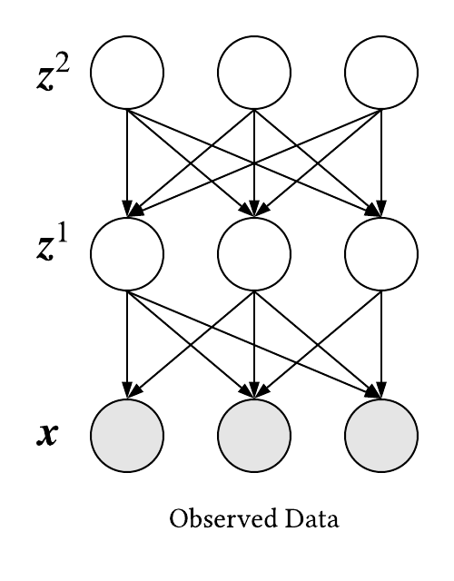
It should be noted (Burda et al., 2016) proposed this architecture which is a mere generalization of the original architecture used in (Kingma and Welling, 2014). The goal is to use maximum likelihood estimation to learn the parameters, \(\boldsymbol{\theta}\), of the following distribution:

There are some underlining takeaways from the above distribution:

• It tends to be intractable because our model assumes \(z_i^l \not\!\perp\!\!\!\perp z_j^l | \ \boldsymbol{x} \ \cup \ \boldsymbol{z^{l-1}} \ \forall \ i \neq j,l \) (explaining away). This requires integration over all combinations our latent variables can take on.
• The probability density functions on the right tends to a traditional distribution, say a Gaussian, but is parameterized by some deep network.

Since our current distribution is intractable, we must resort to variational inference to learn \( \boldsymbol{\theta} \).

3. Variational Inference

If we recall, MLE is a simple optimization problem which returns a set of parameters that maximizes the likelihood that our data came from some distribution of our choice. Our objective function is the log likelihood and variational inference simply replaces this function with a lower bound function (evidence lower bound or ELBO) that is tractable. So, as we learn a set of parameters that maximizes the likelihood of our lower bound we are also increasing the likelihood of our original distribution (this is the definition of a lower bound).

3.1 Deriving the ELBO

The derivation of the lower bound is a mere byproduct of Jensen's Inequality which simply states: for any concave function, \(f,\) we have \( f(\mathbb{E}[u]) \geq \mathbb{E}[f(u)]\). So, we layout the following:

Ignoring \(q_{\boldsymbol{\phi}} \) for a second, all we have done thus far is rewritten our log likelihood function in a clever way. I emphasis clever because we can now invoke Jensen's Inequality where:

Going forward, we will use \(\mathcal{L}(\boldsymbol{x})\) as our objective function of concern where \(q_{\boldsymbol{\phi}} (\boldsymbol{z}|\boldsymbol{x})\) is essentially a surrogate distribution for \(p_{\boldsymbol{\theta}}(\boldsymbol{z|x}) \). Now, we define the following for \(q_{\boldsymbol{\phi}}(\boldsymbol{z}|\boldsymbol{x})\):

This is known as mean field approximation which yields a tractable surrogate distribution.

3.1.1 Making More Sense of the ELBO

Understanding some variations of the ELBO really sheds light on the underlining intuitions of Variational Inference. For starters, we can rewrite the ELBO in the following form:

Note, the second expectation on the third line does not touch \(p_{\boldsymbol{\theta}}(\boldsymbol{x})\) , so it evaluates to 1. Furthermore, we should notice in the last line KL Divergence has made an appearance—which is a non-negative number that quantifies the distance between two distributions; where 0 is returned if the two distributions under concern are identical.

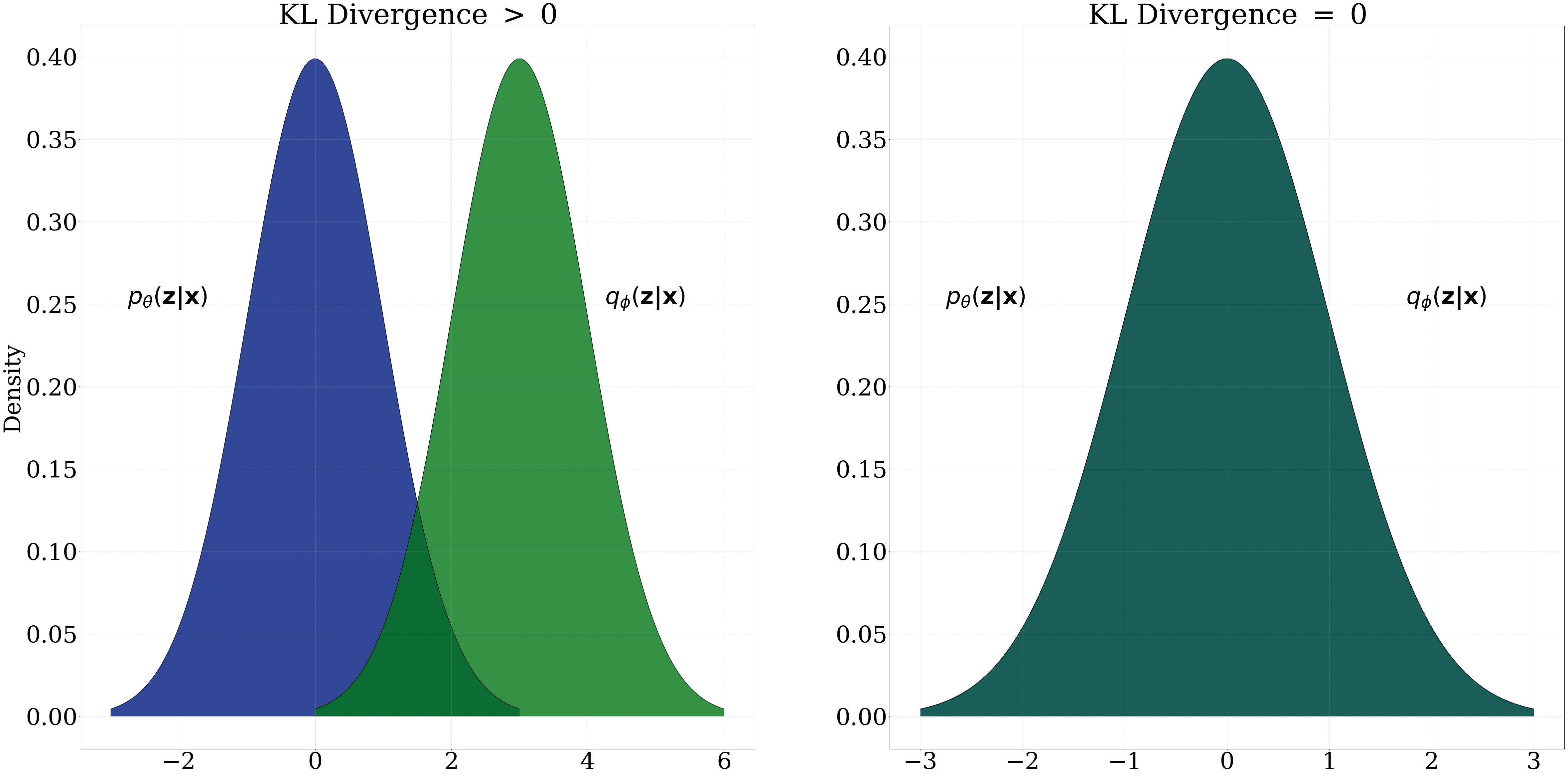
So, maximizing the lower bound is actually maximizing our original log probability and subtracting the distance between the intractable distribution and the surrogate distribution. Theoretically, we could set \( q_{\boldsymbol{\phi}}(\boldsymbol{z|x}) = q_{\boldsymbol{\theta}}(\boldsymbol{z|x}) \) and our lower bound would be tight!

4. Relationship to Autoencoders

Thus far, all we have done is explore the variational component of VAEs by understanding the theoretical properties of the lower bound. Now, we will begin to understand the learning process of VAEs and their relationship to autoencoders.

4.1 Recognition Network

We define the following:

All of the distributions in the Recognition Network are Gaussians parameterized by a mean vector, \(\boldsymbol{\mu}(\cdot)\), and a diagonal covariance matrix, \(\boldsymbol{\Sigma}(\cdot)\). Each of these are deterministic neural networks, e.g., FFNN, CNN or RNN parameterized by \(\boldsymbol{\phi}\). The goal of the recognition network is to take in some observed data point, \(\boldsymbol{x}\), and learn the latent features, \(\boldsymbol{z}\), that best describe our data. In literature this is also known as the encoder network because we are encoding information about \(\boldsymbol{x}\) into \(\boldsymbol{z}\).

4.2 Generative Network

We define the following:

We notice \(p(\boldsymbol{z}^2)\) is just the standard normal distribution and all other distributions are equivalent to the ones in the Recognition Network. The Generative Network uses the latent features to maximize the likelihood over the the joint distribution, \(p_{\boldsymbol{\theta}}(\boldsymbol{x,z})\). After learning, we can sample from \(\boldsymbol{x}_{new} \sim p_{\boldsymbol{\theta}}(\boldsymbol{x}_{observed}|\boldsymbol{z}^1)\) to generate a new example. Note, \(p_{\boldsymbol{\theta}}(\boldsymbol{x}|\boldsymbol{z}^1)\) = \(p_{\boldsymbol{\theta}}(\boldsymbol{x}|\boldsymbol{z}^1, \boldsymbol{z}^2)\) , as defined by our graphical model. In literature this is known as the decoder network because we decode the information in \(\boldsymbol{z}\) to generate a new example, \(\boldsymbol{x}_{new}\).

It should be noted the idea of a recognition and generative network is not new—where Helmholtz Machines, (Dayan, 1995), used an identical architecture but were trained using the Wake-sleep algorithm.

5. The Learning Process

Let us recall the objective function we are trying to maximize:

We want to learn the parameters, \(\boldsymbol{\theta}\text{ and } \boldsymbol{\phi}\) , in an end-to-end fashion. With this at hand, we can layout the computational graph:

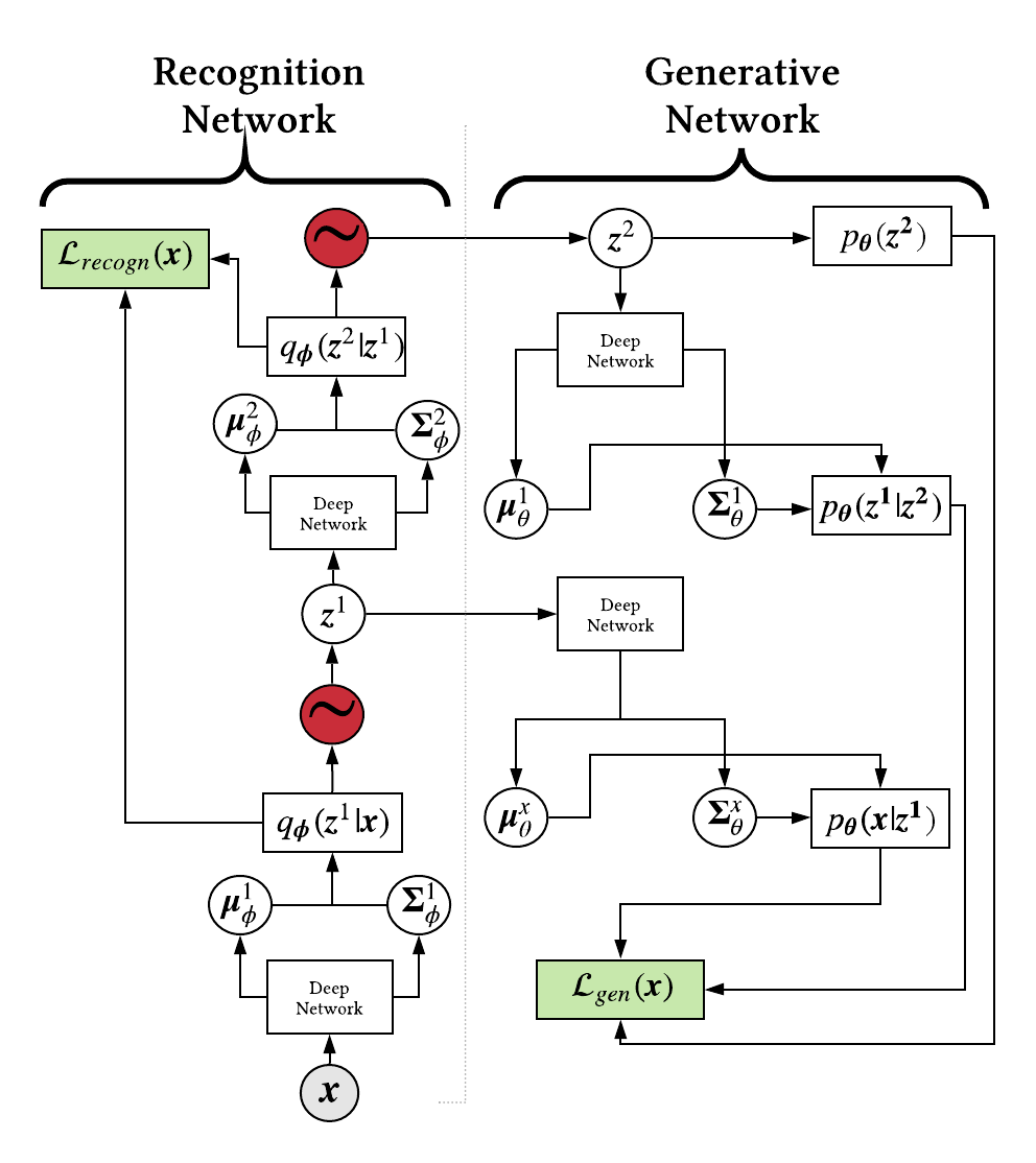
I will acknowledge this may appear overwhelming but I did not fully understand the learning process nor the reparameterization trick until stepping through this graph in its entirety. A forward pass begins, bottom left, by taking an observed data point and sending it through the recognition network. Along the way, we sample a latent vector, \(\boldsymbol{z}^l\), send it through a deep network and generate the next set of parameters for an upstream distribution. After each latent layer has been sampled, we can forward propagate through the generative network.

Back propagation is actually fairly straightforward up until propagating through the latent nodes. Ultimately, the latent variables are stochastic and we cannot differentiate through a stochastic operator, red nodes. As a result, we would have to rely on gradient estimates via MCMC sampling which typically leads to high variance gradients and poor learning.

5.1 Reparameterization Trick

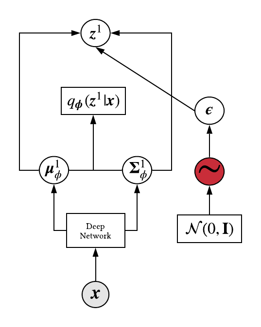
Let us now define \(\boldsymbol{z}^l\) as a deterministic random variable:

$$ \begin{aligned} \boldsymbol{z}^l &= g\bigg(\boldsymbol{\mu}(i,\boldsymbol{\phi}), \boldsymbol{\Sigma}(i,\boldsymbol{\phi}),\boldsymbol{\epsilon}\bigg) \\ &=\boldsymbol{\mu}(i,\boldsymbol{\phi}) + \boldsymbol{\Sigma}(i,\boldsymbol{\phi})^{\frac{1}{2}}\otimes \boldsymbol{\epsilon} && \boldsymbol{\epsilon}\sim \mathcal{N}(0,\textbf{I}) \end{aligned} $$

\(i\) is just an argument and \(\boldsymbol{\Sigma}(i,\boldsymbol{\phi})^{\frac{1}{2}}\) is the standard deviation as opposed to the variance. So, once we sample an \(\boldsymbol{\epsilon}\) from the standard normal we can use it to calculate \(\boldsymbol{z}^l\). Ultimately, the stochasticity now lies in \(\boldsymbol{\epsilon}\) and not in \(\boldsymbol{z}^l\). Also, we can quickly show the reparameterized latent variable still yields the same expected value and variance:

$$ \begin{aligned} \mathbb{E}_{\boldsymbol{\epsilon}\sim\mathcal{N}(0,\textbf{I})} [\boldsymbol{z}^l]&= \boldsymbol{\mu} + \boldsymbol{\Sigma}^{\frac{1}{2}} \mathbb{E}_{\boldsymbol{\epsilon}\sim\mathcal{N}(0,\textbf{I})} [\boldsymbol{\epsilon}] \\ &=\boldsymbol{\mu} + 0 \\ \\ \text{Var}[\boldsymbol{z}^l]&= \mathbb{E}_{\boldsymbol{\epsilon}\sim\mathcal{N}(0,\textbf{I})} \bigg[ \bigg( \boldsymbol{\mu} + \boldsymbol{\Sigma}^{\frac{1}{2}}\boldsymbol{\epsilon} \bigg)^2 \bigg] - \mathbb{E}_{\boldsymbol{\epsilon}\sim\mathcal{N}(0,\textbf{I})} [\boldsymbol{z}^l]^2\\ &= \boldsymbol{\mu}^2 + 2\boldsymbol{\mu}\boldsymbol{\Sigma}^{\frac{1}{2}} \mathbb{E}_{\boldsymbol{\epsilon}\sim\mathcal{N}(0,\textbf{I})} [\boldsymbol{\epsilon}] + \boldsymbol{\Sigma} \mathbb{E}_{\boldsymbol{\epsilon}\sim\mathcal{N}(0,\textbf{I})} [\boldsymbol{\epsilon}^2] - \boldsymbol{\mu}^2 \\ &=\boldsymbol{\Sigma}\textbf{I} \end{aligned} $$

where notation was simplified for brevity.

Now let us update the computational graph.

We can now back propagate through all learnable parameters!

Conclusion

Now that we understand the theory of VAEs, we are in position to train a model and be informed adjudicators of its performance. Luckily, TensorFlow and Jan Hendrik Metzen have great tutorials on programmatic implementations.

Bibliography

Yuri Burda, Roger Grosse, and Ruslan Salakhutdinovz. Impotance weigthed autoenocders. 2016. URL: https://arxiv.org/pdf/1509.00519.pdf. ↩

Peter Dayan. Helholtz machines and wake-sleep learning. Handbook of Brain Theory of Neural Networks, 2., 1995. URL: https://pdfs.semanticscholar.org/dd8c/da00ccb0af1594fbaa5d41ee639d053a9cb2.pdf. ↩

Geoffrey Hinton, Peter Dayan, Brendan J Frey, and Radford M Neal. The wake-sleep alogrithm for unsupervised neural networks. 1995. URL: http://www.cs.toronto.edu/~fritz/absps/ws.pdf. ↩

Diederik Kingma and Max Welling. Auto-encoding variational bayes. 2014. URL: https://arxiv.org/pdf/1312.6114.pdf. ↩ ^{1 2}

Carnegie Mellon University 10-708 Probabilistic Graphical Models Spring 2019

Carnegie Mellon University 10-707 Deep Learning Spring 2019

Lil'Log From Autoencoder to Beta-VAE

---